Posterior Sampling with Conditional Diffusion Models

Author

Elling Svee

Published

September 22, 2026

Many problems in science and engineering are inverse problems. We observe indirect or corrupted measurements and want to recover the unknown quantity that generated them. Examples include recovering a signal from incomplete observations, or inferring physical parameters from experimental data. These problems are often ill-posed, meaning that many different solutions may be consistent with the observations. A natural way to handle this ambiguity is through Bayesian inference. Let \(\boldsymbol{x}\) denote the unknown quantity and \(\boldsymbol{y}\) the observed data. Bayes’ rule gives

\[ p(\boldsymbol{x} \mid \boldsymbol{y}) \propto p(\boldsymbol{y} \mid \boldsymbol{x})\,p(\boldsymbol{x}), \]

where:

Prior \(p(\boldsymbol{x})\): describes what solutions are plausible before observing the data.
Likelihood \(p(\boldsymbol{y} \mid \boldsymbol{x})\): describes the measurement process and how well a candidate \(\boldsymbol{x}\) explains the observations.
Posterior \(p(\boldsymbol{x} \mid \boldsymbol{y})\): combines both sources of information and represents our uncertainty about \(\boldsymbol{x}\) after observing \(\boldsymbol{y}\).

The challenge is that useful priors for high-dimensional objects are difficult to specify explicitly. Generative diffusion models provide an attractive alternative. Here, a diffusion model trained on representative data can act as a learned prior. Instead of restricting solutions using a hand-designed regularizer, the model captures complex structure directly from data. By combining this learned prior with the likelihood during the diffusion sampling process, we can approximately sample from the posterior without retraining the generative model for every new inverse problem.

Benefits of using diffusion models as priors include:

Expressive priors: Can capture complex, high-dimensional distributions that are difficult to model analytically.
Reusable prior: A pretrained diffusion model can be combined with different forward models and likelihoods without retraining.
High-dimensional inference: Can handle high-dimensional inverse problems where traditional methods may struggle.

However, compared to approaches like MCMC or variational inference, there are also some limitations:

Computational cost: Posterior sampling may require many neural-network evaluations. There are ways to reduce this, like flow-based methods, but this is not discussed here. Scaling to very high-dimensional problems may also require additional techniques, such as generating lower-dimensional latent representations, to make the problem tractable.
Approximate inference: Methods such as DPS generally do not produce exact posterior samples and may introduce bias. However, we will explore ways to address this.
Prior mismatch: If the true solution differs substantially from the diffusion model’s training distribution, the prior can lead to misleading reconstructions.
Limited interpretability: A learned generative prior is harder to understand and analyze than simple analytical priors.

This post gives an overview of the main ideas behind diffusion models, and how they can be used for posterior sampling in inverse problems. We rely on the score-based diffusion framework for a clean theoretical foundation (Song et al. 2021), and our notation and explanations are inspired by a book called The Principles of Diffusion Models (Lai et al. 2025).

from typing import Callable, NamedTuple

import jax.numpy as jnp
import jax.random as random
import jax.scipy.stats as stats
import optax
from flax import nnx
from jax import Array, grad, vmap
from jax.nn import softmax
import matplotlib.pyplot as plt

# Style and color settings for plots
plt.style.use("tableau-colorblind10")
plt.rcParams.update(
    {
        "text.usetex": False,
        "font.family": "monospace",
        "font.monospace": ["Lucida Console", "DejaVu Sans Mono"],
        "font.size": 14,
        "mathtext.fontset": "custom",
        "mathtext.rm": "DejaVu Sans Mono",
        "mathtext.it": "DejaVu Sans Mono:italic",
        "mathtext.bf": "DejaVu Sans Mono:bold",
    }
)

THEME_COLORS = plt.rcParams["axes.prop_cycle"].by_key()["color"]
PLOT_COLORS = {
    "prior": "black",
    "likelihood": THEME_COLORS[5],
    "posterior": THEME_COLORS[0],
    "samples": THEME_COLORS[6],
    "loss": "black",
}
COLORBAR_PAD = 0.02

Problem setup

We consider a deliberately simple one-dimensional inverse problem in which all relevant distributions can be computed analytically. This gives us a ground truth against which we can compare the diffusion-based posterior samplers later in the post. The setup is adapted from the Gaussian-mixture example on page 24 of these lecture notes.

The unknown state is a scalar \(x\in\mathbb{R}\). We assign it a three-component Gaussian-mixture prior, \[ p(x)=\sum_{k=1}^3 w_k\,\mathcal{N}(x;\mu_k,\sigma_k^2), \] with component weights, means, and standard deviations \[ \mathbf{w}=(0.3,0.5,0.2),\qquad \boldsymbol{\mu}=(-2.5,0,1.5),\qquad \boldsymbol{\sigma}=(0.3,0.4,0.3). \] The separated modes make the prior simple enough to visualize, while retaining the multimodality that makes posterior guidance challenging. We observe the state through the identity forward operator with additive Gaussian noise, \[ y=x+\eta,\qquad \eta\sim\mathcal{N}(0,\sigma_y^2). \] giving the likelihood is \(p(y\mid x)=\mathcal{N}(y;x,\sigma_y^2)\). We use the observation \(y_{\mathrm{obs}}=0.5\) and noise standard deviation \(\sigma_y=0.8\). Bayes’ rule then gives

\[ p(x\mid y_{\mathrm{obs}}) =\frac{p(y_{\mathrm{obs}}\mid x)p(x)}{p(y_{\mathrm{obs}})}. \]

Because both the likelihood and each prior component are Gaussian, the posterior is also a three-component Gaussian mixture. For component \(k\), Gaussian conditioning gives

\[ \widetilde{\sigma}_k^2 =\left(\frac{1}{\sigma_k^2}+\frac{1}{\sigma_y^2}\right)^{-1} =\frac{\sigma_k^2\sigma_y^2}{\sigma_k^2+\sigma_y^2}, \qquad \widetilde{\mu}_k =\widetilde{\sigma}_k^2 \left(\frac{\mu_k}{\sigma_k^2} +\frac{y_{\mathrm{obs}}}{\sigma_y^2}\right), \]

while the component weights are updated according to their evidence,

\[ \widetilde{w}_k =\frac{ w_k\,\mathcal{N}(y_{\mathrm{obs}};\mu_k,\sigma_k^2+\sigma_y^2) }{ \sum_{j=1}^3 w_j\,\mathcal{N}(y_{\mathrm{obs}};\mu_j,\sigma_j^2+\sigma_y^2) }. \]

For our chosen observation, the posterior weights are approximately \((0.0012,0.8011,0.1977)\). The likelihood therefore almost eliminates the leftmost prior mode at \(x=-2.5\), while preserving posterior mass around both remaining modes. This analytically available posterior will serve as the reference distribution in our experiments.

class GaussianMixture(NamedTuple):
    weights: Array
    means: Array
    stds: Array


def mixture_density(x: Array, mixture: GaussianMixture) -> Array:
    return jnp.sum(
        mixture.weights * stats.norm.pdf(x[..., None], mixture.means, mixture.stds),
        axis=-1,
    )


def mixture_score(x: Array, mixture: GaussianMixture) -> Array:
    log_component_densities = jnp.log(mixture.weights) + stats.norm.logpdf(
        x[..., None], mixture.means, mixture.stds
    )
    responsibilities = softmax(log_component_densities, axis=-1)
    component_scores = -(x[..., None] - mixture.means) / mixture.stds**2
    return jnp.sum(responsibilities * component_scores, axis=-1)


def sample_mixture(key: Array, mixture: GaussianMixture, num_samples: int) -> Array:
    component_key, noise_key = random.split(key)
    components = random.categorical(
        component_key, jnp.log(mixture.weights), shape=(num_samples,)
    )
    noise = random.normal(noise_key, shape=(num_samples,))
    return mixture.means[components] + mixture.stds[components] * noise


def likelihood_density(x: Array, observation: float, observation_std: float) -> Array:
    return stats.norm.pdf(observation, x, observation_std)


def condition_mixture(
    prior: GaussianMixture, observation: float, observation_std: float
) -> GaussianMixture:
    posterior_variance = 1 / (1 / prior.stds**2 + 1 / observation_std**2)
    posterior_means = posterior_variance * (
        prior.means / prior.stds**2 + observation / observation_std**2
    )
    unnormalised_weights = prior.weights * stats.norm.pdf(
        observation, prior.means, jnp.sqrt(prior.stds**2 + observation_std**2)
    )
    posterior_weights = unnormalised_weights / jnp.sum(unnormalised_weights)
    return GaussianMixture(
        posterior_weights,
        posterior_means,
        jnp.sqrt(posterior_variance),
    )

grid = jnp.linspace(-4, 4, 1_000)
prior_mixture = GaussianMixture(
    weights=jnp.array([0.3, 0.5, 0.2]),
    means=jnp.array([-2.5, 0.0, 1.5]),
    stds=jnp.array([0.3, 0.4, 0.3]),
)
observation = 0.5
observation_std = 0.8
posterior_mixture = condition_mixture(prior_mixture, observation, observation_std)

prior_density = mixture_density(grid, prior_mixture)
likelihood = likelihood_density(grid, observation, observation_std)
posterior_density = mixture_density(grid, posterior_mixture)

fig, ax = plt.subplots(figsize=(10, 6))
ax.plot(grid, prior_density, label="Prior", color=PLOT_COLORS["prior"], linewidth=3)
ax.plot(
    grid,
    likelihood,
    label="Likelihood",
    color=PLOT_COLORS["likelihood"],
    linewidth=3,
)
ax.plot(
    grid,
    posterior_density,
    label="Posterior",
    color=PLOT_COLORS["posterior"],
    linewidth=3,
)
ax.set(xlabel="State", ylabel="Density")
ax.legend()
fig.tight_layout()
plt.show()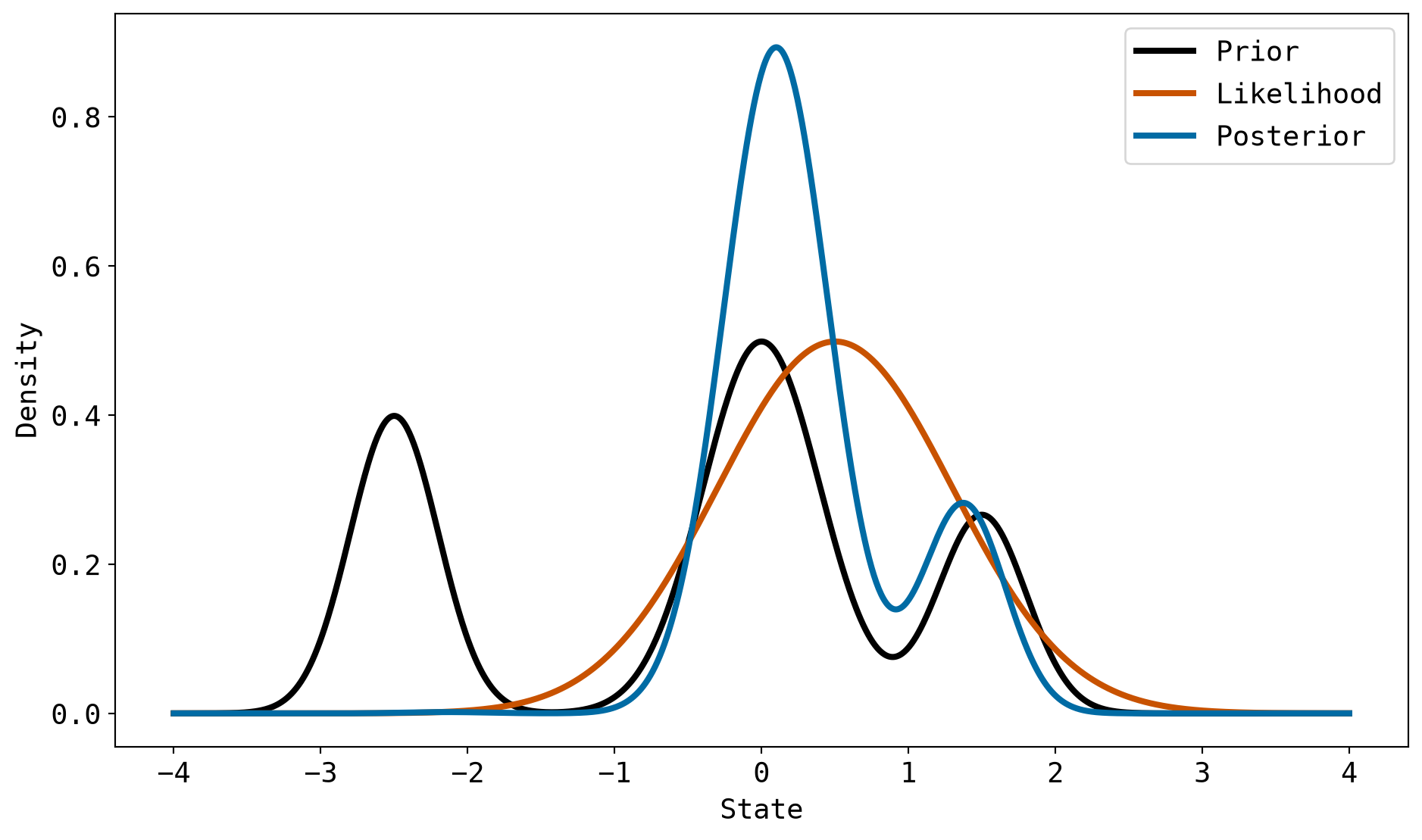

Prior sampling using a generative diffusion model

A diffusion model learns a mapping from pure Gaussian noise to a target distribution. Instead of learning this mapping directly, the model is trained to denoise a progressively corrupted version of the target distribution. Formally, the diffusion model is defined through a continuous-time stochastic process \(\mathbf{x}(t)\) governed by a forward stochastic differential equation (SDE) on the interval \([0,T]\): \[ \mathrm{d}\mathbf{x}(t) = \mathbf{f}(\mathbf{x}(t),t)\,\mathrm{d}t + g(t)\,\mathrm{d}\mathbf{w}(t), \qquad \mathbf{x}(0) \sim p_0. \tag{1}\] Here \(\mathbf{f}(\cdot,t):\mathbb{R}^D\to\mathbb{R}^D\) is the drift, \(g(t)\in\mathbb{R}\) is the scalar diffusion coefficient, and \(\mathbf{w}(t)\) denotes a standard Wiener process. Without too much rigour, a Wiener process is a continuous-time stochastic process that starts at zero, has independent increments, and satisfies that for any \(s<t\), the increment \(\mathbf{w}(t)-\mathbf{w}(s)\) is normally distributed with mean zero and variance \(t-s\).

Once \(\mathbf{f}\) and \(g\) are specified, the forward process is fully determined, describing how the data is progressively corrupted through the injection of Gaussian noise. For this post, we focus on a variance-preserving SDE, where \[ \mathbf{f}(\mathbf{x},t)=-\frac{1}{2}\beta(t)\mathbf{x}, \qquad g(t)=\sqrt{\beta(t)}, \] with a linear schedule \(\beta(t)=\beta_{\min}+\frac{t}{T}(\beta_{\max}-\beta_{\min})\) for some \(0<\beta_{\min}<\beta_{\max}\). At the end of the forward process, the distribution of \(\mathbf{x}(T) \sim p_T \approx \mathcal{N}(0,I)\), regardless of the initial distribution \(p_0\). Discretizing Equation 1 with the Euler–Maruyama method for a small time step \(\Delta t\) gives the update rule

\[ \mathbf{x}_{t+\Delta t} = \mathbf{x}_t-\frac{1}{2}\beta(t)\mathbf{x}_t\Delta t +\sqrt{\beta(t)\Delta t}\,\boldsymbol{\epsilon}_t, \qquad \boldsymbol{\epsilon}_t\sim\mathcal{N}(0,I). \] Although the proof is not provided here, we can also derive the distribution of \(\mathbf{x}_t\mid\mathbf{x}_0\). Denoting \[ \alpha_t = \exp\!\left(-\frac{1}{2}\int_0^t\beta(\tau)\,\mathrm{d}\tau\right) \quad\text{and}\quad \sigma_t^2 = 1-\alpha_t^2, \] the Gaussian corruption kernel can be expressed as \(\mathbf{x}_t = \alpha_t\mathbf{x}_0 + \sigma_t\boldsymbol{\epsilon}\) with \(\boldsymbol{\epsilon}\sim\mathcal{N}(0,I)\), which gives the conditional distribution \[ p_t(\mathbf{x}_t\mid\mathbf{x}_0) =\mathcal{N}\!\left( \mathbf{x}_t; \alpha_{t}\mathbf{x}_0, \sigma_t^2\mathbf{I} \right). \tag{2}\]

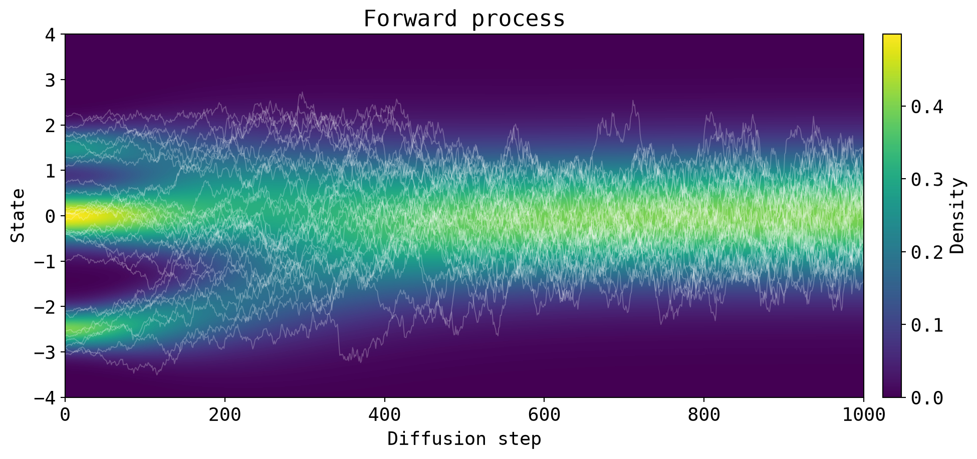
This is useful because it allows us to sample from the forward process at any time \(t\) without simulating the entire trajectory from \(0\) to \(t\).

The following plot illustrates how the forward process transforms the prior distribution to a simple Gaussian distribution as \(t\) approaches \(T\). We plot the distribution over time as a heatmap, with some example trajectories of the forward process on top.

def linear_beta_schedule(
    num_steps: int, beta_start: float = 1e-4, beta_end: float = 0.02
) -> Array:
    return jnp.linspace(beta_start, beta_end, num_steps)


def f(x: Array, beta_t: float) -> Array:
    return -0.5 * beta_t * x


def g(beta_t: float) -> Array:
    return jnp.sqrt(beta_t)


def forward_step(x: Array, dt: float, beta_t: float, key: Array) -> Array:
    epsilon = random.normal(key, shape=x.shape)
    return x + f(x, beta_t) * dt + g(beta_t) * jnp.sqrt(dt) * epsilon


def diffuse_mixture(
    mixture: GaussianMixture, integrated_beta: Array
) -> GaussianMixture:
    exp_integrated_beta = jnp.exp(-integrated_beta)
    return GaussianMixture(
        mixture.weights,
        jnp.sqrt(exp_integrated_beta) * mixture.means,
        jnp.sqrt(exp_integrated_beta * mixture.stds**2 + (1 - exp_integrated_beta)),
    )


def sample_forward_process(
    key: Array,
    initial_samples: Array,
    betas: Array,
    dt: float,
) -> tuple[Array, Array]:
    samples = initial_samples
    trajectories = [samples]
    for beta_t in betas:
        key, step_key = random.split(key)
        samples = forward_step(samples, dt, beta_t, step_key)
        trajectories.append(samples)
    return key, jnp.stack(trajectories)

num_steps = 1000
num_samples = 30_000
dt = 1.0
betas = linear_beta_schedule(num_steps)
integrated_betas = jnp.concatenate((jnp.zeros(1), jnp.cumsum(betas * dt)))

key = random.key(0)
key, sample_key = random.split(key)
initial_samples = sample_mixture(sample_key, prior_mixture, num_samples)
key, forward_trajectories = sample_forward_process(key, initial_samples, betas, dt)

diffused_prior_mixtures = vmap(diffuse_mixture, in_axes=(None, 0))(
    prior_mixture, integrated_betas
)
prior_density_by_time = vmap(mixture_density, in_axes=(None, 0))(
    grid, diffused_prior_mixtures
)

def plot_trajectories(
    trajectories: Array,
    density_by_time: Array,
    title: str,
) -> None:
    num_steps, num_samples = trajectories.shape[0] - 1, trajectories.shape[1]
    trajectory_indices = jnp.linspace(0, num_samples - 1, 30, dtype=jnp.int32)
    fig, ax = plt.subplots(figsize=(11, 5))
    image = ax.imshow(
        density_by_time.T,
        origin="lower",
        aspect="auto",
        cmap="viridis",
        extent=(0, num_steps, float(grid[0]), float(grid[-1])),
    )
    ax.grid(False)
    ax.plot(
        jnp.arange(num_steps + 1),
        trajectories[:, trajectory_indices],
        color="white",
        alpha=0.25,
        linewidth=0.7,
    )
    fig.colorbar(image, ax=ax, pad=COLORBAR_PAD, label="Density")
    ax.set(xlabel="Diffusion step", ylabel="State", title=title)
    fig.tight_layout()
    plt.show()


def plot_reverse_samples(
    trajectories: Array,
    density_by_time: Array,
    target_density: Array,
    trajectory_title: str,
    histogram_title: str,
    target_label: str,
    sample_weights: Array | None = None,
) -> None:
    num_steps, num_samples = trajectories.shape[0] - 1, trajectories.shape[1]
    trajectory_indices = jnp.linspace(0, num_samples - 1, 30, dtype=jnp.int32)
    fig, axes = plt.subplots(1, 2, figsize=(16, 5))
    image = axes[0].imshow(
        density_by_time.T,
        origin="lower",
        aspect="auto",
        cmap="viridis",
        extent=(0, num_steps, float(grid[0]), float(grid[-1])),
    )
    axes[0].grid(False)
    axes[0].plot(
        jnp.arange(num_steps + 1),
        trajectories[:, trajectory_indices],
        color="white",
        alpha=0.25,
        linewidth=0.7,
    )
    fig.colorbar(image, ax=axes[0], pad=COLORBAR_PAD, label="Density")
    axes[0].set(
        xlabel="Diffusion step",
        ylabel="State",
        title=trajectory_title,
    )
    axes[1].hist(
        trajectories[0],
        bins=60,
        range=(float(grid[0]), float(grid[-1])),
        density=True,
        weights=sample_weights,
        color=PLOT_COLORS["samples"],
        edgecolor="white",
        label="Samples",
    )
    axes[1].plot(
        grid,
        target_density,
        color=PLOT_COLORS[target_label.lower()],
        linewidth=3,
        label=target_label,
    )
    axes[1].set(xlabel="State", ylabel="Density", title=histogram_title)
    axes[1].legend()
    fig.tight_layout()
    plt.show()


plot_trajectories(
    forward_trajectories,
    prior_density_by_time,
    "Forward process",
)

Intuitively, we can imagine that if we could run the forward process backwards, we would be able to start from pure noise and recover samples from the prior distribution. The insight of score-based diffusion models is that, although we cannot reverse individual stochastic trajectories, the distribution over those trajectories is reversible. Anderson (1982) formalizes this by constructing a time-reversed process \(\widetilde{\mathbf{x}}(t)\) defined by the SDE

\[ \begin{aligned} \mathrm{d}\widetilde{\mathbf{x}}(t) &=\left[\mathbf{f}(\widetilde{\mathbf{x}}(t),t) -g^2(t)\nabla_{\mathbf{x}}\log p_t(\widetilde{\mathbf{x}}(t))\right]\mathrm{d}t +g(t)\,\mathrm{d}\widetilde{\mathbf{w}}(t), \end{aligned} \tag{3}\]

Here \(\widetilde{\mathbf{w}}(t)\) denotes a standard Wiener process in reverse time, defined as \(\widetilde{\mathbf{w}}(t)=\mathbf{w}(T-t)-\mathbf{w}(T)\). Those familiar with MCMC might also notice the similarity to Langevin dynamics used in the MALA algorithm (Dunson and Johndrow 2020), where the score function \(\nabla_{\mathbf{x}}\log p_t\) is used to guide the process towards regions of high probability. Discretizing Equation 3 in a similar manner as for the forward process yields the stochastic updates

\[ \begin{aligned} \widetilde{\mathbf{x}}_{t-\Delta t} ={}&\widetilde{\mathbf{x}}_t -\left[-\frac{1}{2}\beta(t)\widetilde{\mathbf{x}}_t -\beta(t)\nabla_{\widetilde{\mathbf{x}}_t}\log p_t(\widetilde{\mathbf{x}}_t)\right]\Delta t -\sqrt{\beta(t)\Delta t}\,\widetilde{\boldsymbol{\epsilon}}_t, \quad \widetilde{\boldsymbol{\epsilon}}_t\sim\mathcal{N}(0,\mathbf{I}). \end{aligned} \tag{4}\]

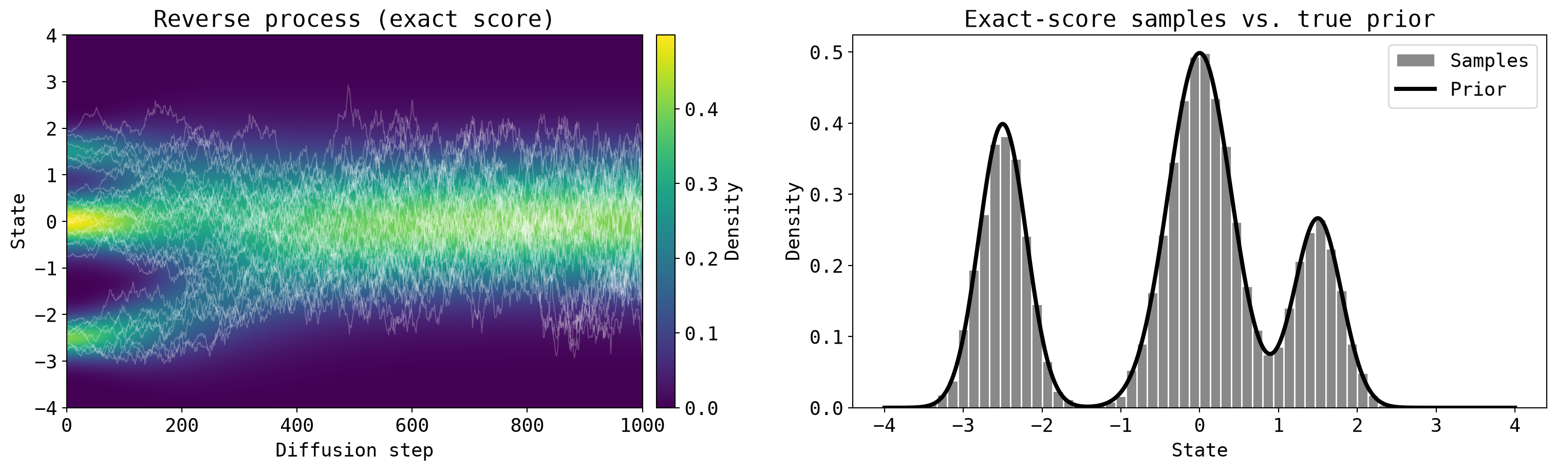
Observe that the score \(\nabla_{\mathbf{x}}\log p_t\) is the only term that depends on the unknown distribution \(p_t\). If we knew it for all \(t\), we could sample from \(p_0\) by starting from \(p_T\approx \mathcal{N}(\mathbf{0},\mathbf{I})\) and iteratively applying the updates above. For our simple multimodal example, we can compute the score function analytically, allowing us to do exactly that. The following plot shows the resulting samples from the prior distribution, which match the ground truth distribution very closely.

def reverse_step(x: Array, dt: float, beta_t: float, score: Array, key: Array) -> Array:
    epsilon = random.normal(key, shape=x.shape)
    drift = f(x, beta_t) - g(beta_t) ** 2 * score
    return x - drift * dt + g(beta_t) * jnp.sqrt(dt) * epsilon


def sample_reverse_process(
    key: Array,
    initial_samples: Array,
    betas: Array,
    dt: float,
    score_function: Callable[[Array, int], Array],
) -> tuple[Array, Array]:
    num_steps = len(betas)
    samples = initial_samples
    trajectories = [samples]
    for i in range(num_steps, 0, -1):
        score = score_function(samples, i)
        key, step_key = random.split(key)
        samples = reverse_step(samples, dt, betas[i - 1], score, step_key)
        trajectories.append(samples)
    return key, jnp.stack(trajectories[::-1])

def exact_prior_score(x_t: Array, i: int) -> Array:
    mixture_t = GaussianMixture(
        diffused_prior_mixtures.weights[i],
        diffused_prior_mixtures.means[i],
        diffused_prior_mixtures.stds[i],
    )
    return mixture_score(x_t, mixture_t)


key, initial_key = random.split(key)
initial_samples = random.normal(initial_key, shape=(num_samples,))
key, exact_prior_trajectories = sample_reverse_process(
    key,
    initial_samples,
    betas,
    dt,
    exact_prior_score,
)

plot_reverse_samples(
    exact_prior_trajectories,
    prior_density_by_time,
    prior_density,
    "Reverse process (exact score)",
    "Exact-score samples vs. true prior",
    "Prior",
)

However, in practice we do not have access to the score function and must instead learn it from data. This is done by training a neural-network approximation \(\mathbf{s}_{\boldsymbol{\theta}}(\mathbf{x},t)\approx\nabla_{\mathbf{x}}\log p_t(\mathbf{x})\) to minimize the objective

\[ \mathcal{L}_{\mathrm{SM}}(\boldsymbol{\theta}) = \frac{1}{2} \mathbb{E}_{t\sim\mathcal{U}[0,T]} \mathbb{E}_{\mathbf{x}_t\sim p_t} \left[ \left\| \mathbf{s}_{\boldsymbol{\theta}}(\mathbf{x}_t,t) - \nabla_{\mathbf{x}_t}\log p_t(\mathbf{x}_t) \right\|_2^2 \right]. \]

Since the marginal score \(\nabla_{\mathbf{x}_t}\log p_t(\mathbf{x}_t)\) is generally intractable, we instead rely on the conditional score \(\nabla_{\mathbf{x}_t}\log p_t(\mathbf{x}_t\mid\mathbf{x}_0)\), which is known analytically from Equation 2. In particular, minimizing the denoising score matching objective

\[ \mathcal{L}_{\mathrm{DSM}}(\boldsymbol{\theta}) = \frac{1}{2} \mathbb{E}_{t\sim\mathcal{U}[0,T]} \mathbb{E}_{\mathbf{x}_0} \mathbb{E}_{\mathbf{x}_t\sim p_t(\mathbf{x}_t\mid\mathbf{x}_0)} \left[ \left\| \mathbf{s}_{\boldsymbol{\theta}}(\mathbf{x}_t,t) - \nabla_{\mathbf{x}_t}\log p_t(\mathbf{x}_t\mid\mathbf{x}_0) \right\|_2^2 \right] \]

has the same minimizer as the original score-matching objective, up to a term that is independent of \(\boldsymbol{\theta}\).

Rather than learning the score function directly, it is common to parameterize the model in terms of the noise added by the forward process. In practice, this is often more stable and easier to optimize. For this Gaussian corruption kernel, the conditional score is

\[ \begin{aligned} \nabla_{\mathbf{x}_t} \log p_t(\mathbf{x}_t\mid\mathbf{x}_0) = -\frac{\mathbf{x}_t-\alpha_t\mathbf{x}_0}{\sigma_t^2} = -\frac{\boldsymbol{\epsilon}}{\sigma_t}. \end{aligned} \]

Consequently, a noise-prediction network \(\boldsymbol{\epsilon}_{\boldsymbol{\theta}}(\mathbf{x}_t,t)\) induces the score parameterization

\[ \mathbf{s}_{\boldsymbol{\theta}}(\mathbf{x}_t,t) = -\frac{1}{\sigma_t} \boldsymbol{\epsilon}_{\boldsymbol{\theta}}(\mathbf{x}_t,t). \]

Substituting this parameterization into the denoising score-matching objective gives

\[ \mathcal{L}_{\mathrm{DSM}}(\boldsymbol{\theta}) = \frac{1}{2} \mathbb{E}_{t\sim\mathcal{U}[0,T]} \mathbb{E}_{\mathbf{x}_0} \mathbb{E}_{\boldsymbol{\epsilon}\sim\mathcal{N}(\mathbf{0},\mathbf{I})} \left[ \frac{1}{\sigma_t^2} \left\| \boldsymbol{\epsilon}_{\boldsymbol{\theta}} \left( \alpha_t\mathbf{x}_0+\sigma_t\boldsymbol{\epsilon},t \right) - \boldsymbol{\epsilon} \right\|_2^2 \right]. \] In the following code, we learn the score function through this noise-prediction parameterization using a simple multilayer perceptron with two hidden layers. The neural network is implemented in JAX using the Flax library and trained using the Adam optimizer from Optax.

class MLP(nnx.Module):
    def __init__(self, hidden_sizes: tuple[int, ...], *, rngs: nnx.Rngs):
        sizes = (2,) + hidden_sizes
        self.hidden_layers = nnx.List(
            [
                nnx.Linear(input_size, output_size, rngs=rngs)
                for input_size, output_size in zip(sizes[:-1], sizes[1:], strict=True)
            ]
        )
        self.output_layer = nnx.Linear(hidden_sizes[-1], 1, rngs=rngs)

    def __call__(self, values: Array, times: Array) -> Array:
        hidden = jnp.stack((values, times), axis=-1)
        for layer in self.hidden_layers:
            hidden = nnx.silu(layer(hidden))
        return self.output_layer(hidden)[:, 0]


def denoising_score_matching_loss(
    model: MLP,
    x_0: Array,
    integrated_betas: Array,
    key: Array,
) -> Array:
    step_key, noise_key = random.split(key)
    num_steps = len(integrated_betas) - 1
    steps = random.randint(step_key, x_0.shape, 1, num_steps + 1)
    exp_integrated_beta = jnp.exp(-integrated_betas[steps])
    mean = jnp.sqrt(exp_integrated_beta) * x_0
    variance = 1 - exp_integrated_beta
    epsilon = random.normal(noise_key, x_0.shape)
    x_t = mean + jnp.sqrt(variance) * epsilon
    predicted_epsilon = model(x_t, steps / num_steps)
    return jnp.mean((1 / variance) * jnp.linalg.norm(predicted_epsilon - epsilon) ** 2)


@nnx.jit
def train_step(
    model: MLP,
    optimizer: nnx.Optimizer,
    x_0: Array,
    integrated_betas: Array,
    key: Array,
) -> Array:
    loss, gradients = nnx.value_and_grad(denoising_score_matching_loss)(
        model, x_0, integrated_betas, key
    )
    optimizer.update(model, gradients)
    return loss

steps: int = 30_000
batch_size: int = 512
learning_rate: float = 3e-4

model = MLP((128, 128), rngs=nnx.Rngs(0))
learning_rate = optax.cosine_decay_schedule(learning_rate, steps)
optimizer = nnx.Optimizer(model, optax.adam(learning_rate), wrt=nnx.Param)

key = random.key(1)
losses = []
for _ in range(steps):
    key, batch_key, loss_key = random.split(key, 3)
    x_0 = sample_mixture(batch_key, prior_mixture, batch_size)
    losses.append(train_step(model, optimizer, x_0, integrated_betas, loss_key))
losses = jnp.stack(losses)

fig, ax = plt.subplots(figsize=(8, 4))
ax.plot(losses, color=PLOT_COLORS["loss"])
ax.set(xlabel="Step", ylabel="Loss", yscale="log")
fig.tight_layout()
plt.show()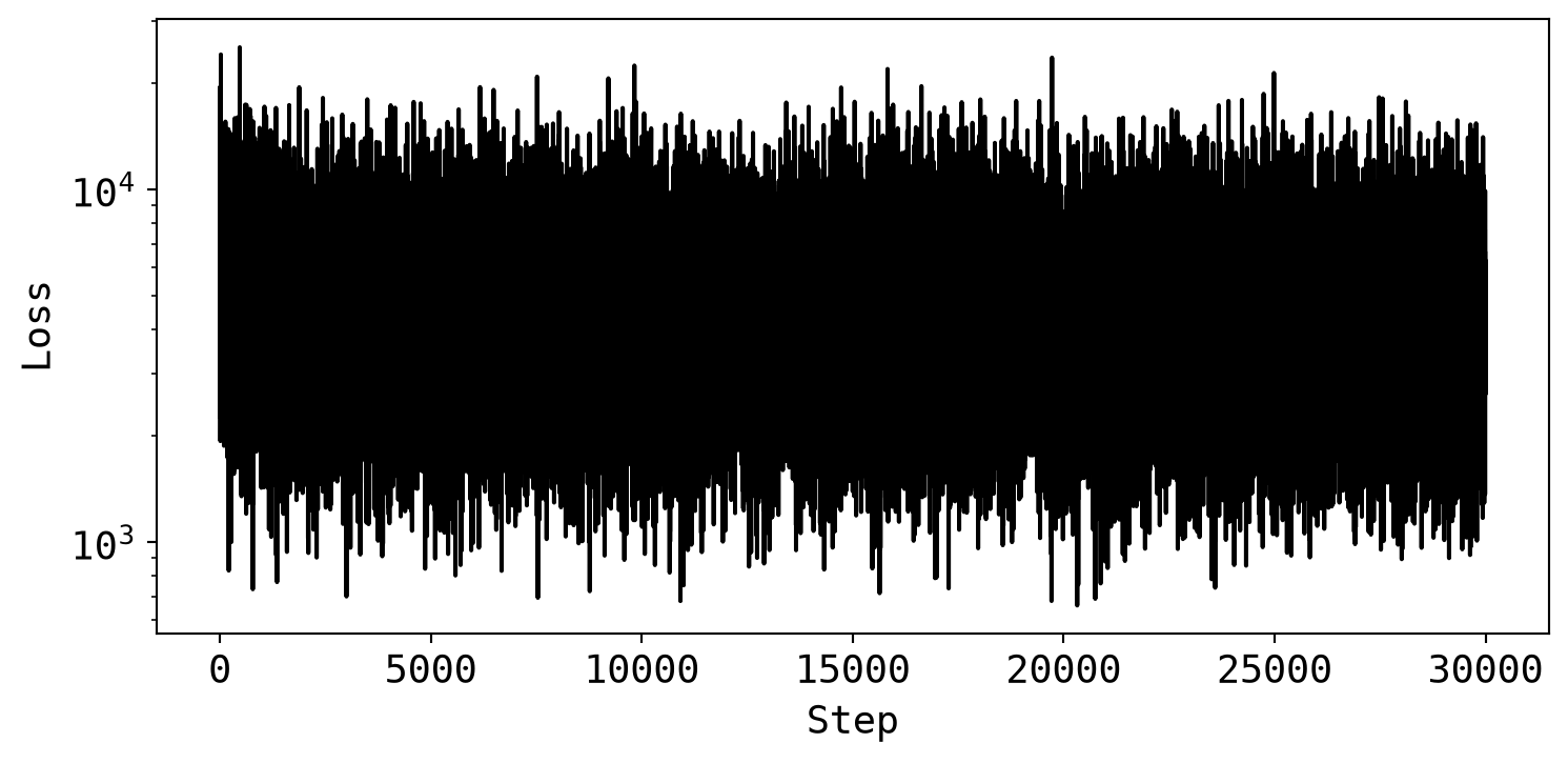

Having learned the score function, we can now sample from the prior distribution using Equation 3. The following illustrates the reverse process and compares the learned and true prior distributions.

def learned_score(
    model: MLP,
    x_t: Array,
    i: int,
    integrated_betas: Array,
) -> Array:
    variance = 1 - jnp.exp(-integrated_betas[i])
    time = jnp.full(x_t.shape, i / (len(integrated_betas) - 1))
    predicted_epsilon = model(x_t, time)
    return -predicted_epsilon / jnp.sqrt(variance)


def learned_prior_score(x_t: Array, i: int) -> Array:
    return learned_score(model, x_t, i, integrated_betas)


key, initial_key = random.split(key)
initial_samples = random.normal(initial_key, shape=(num_samples,))
key, learned_prior_trajectories = sample_reverse_process(
    key,
    initial_samples,
    betas,
    dt,
    learned_prior_score,
)

plot_reverse_samples(
    learned_prior_trajectories,
    prior_density_by_time,
    prior_density,
    "Reverse process (learned score)",
    "Samples vs. true prior",
    "Prior",
)

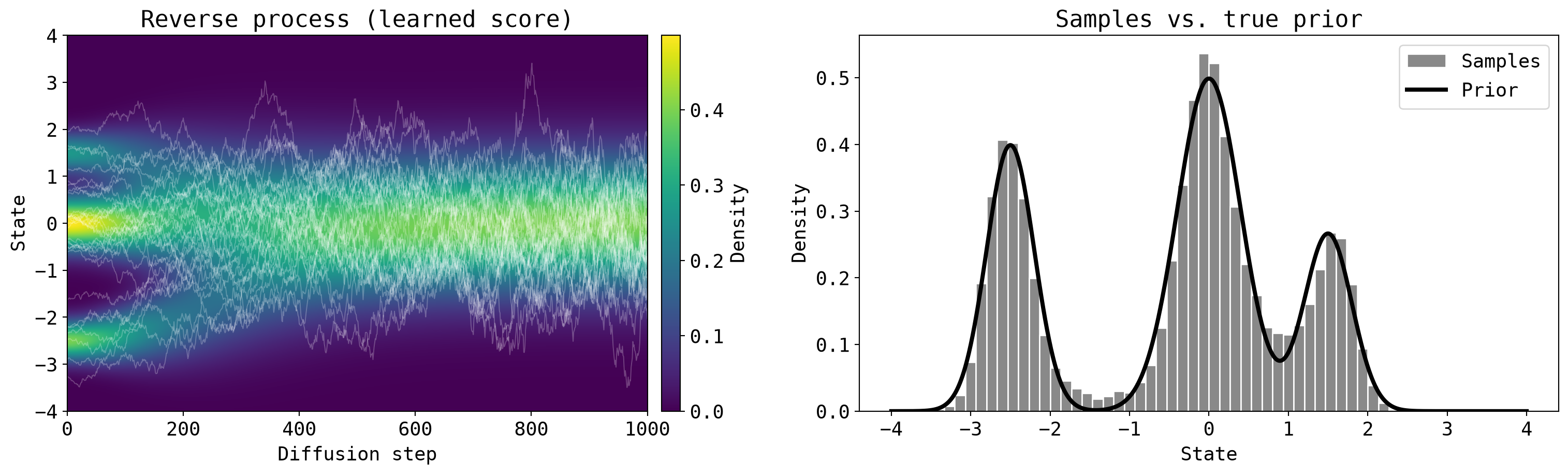
Again, we see that the learned prior distribution matches the ground truth very closely, indicating that the score function has been learned successfully. We can now utilize this learned prior to sample from the posterior distribution.

Sampling from the posterior using training-free guidance

Traditional guidance methods for diffusion models rely on training a separate conditional model to learn the posterior distribution. However, we want to use the learned generative model for the prior directly. Such a training-free approach means that we avoid the need to retrain the model when the conditioning information changes.

To understand how we can use the learned prior model to sample from the posterior, we decompose the posterior score using Bayes’ rule:

\[ \nabla_{\mathbf{x}_t}\log p_t(\mathbf{x}_t\mid\mathbf{y}) = \underbrace{\nabla_{\mathbf{x}_t}\log p_t(\mathbf{x}_t)}_{\text{Prior score}} + \underbrace{\nabla_{\mathbf{x}_t}\log p_t(\mathbf{y}\mid\mathbf{x}_t)}_{\text{Measurement alignment}}. \tag{5}\]

The prior score is what we have already approximated using \(\mathbf{s}_{\boldsymbol{\theta}}(\mathbf{x}_t,t)\), but the measurement-alignment term is generally intractable because it requires marginalizing over the unknown clean sample \(\mathbf{x}_0\). Training-free guidance methods therefore rely on approximating \(\nabla_{\mathbf{x}_t}\log p_t(\mathbf{y}\mid\mathbf{x}_t)\). Once an approximation of the posterior score is available, it can be substituted into the reverse SDE to guide the reverse diffusion process toward the posterior distribution.

Diffusion Posterior Sampling

A commonly used training-free guidance method is Diffusion Posterior Sampling (DPS) (Chung et al. 2024). DPS approximates the measurement alignment by assuming that the conditional distribution \(p(\mathbf{x}_0\mid\mathbf{x}_t)\) is concentrated around its conditional mean. We have

\[ \begin{aligned} p_t(\mathbf{y}\mid\mathbf{x}_t) = \int p(\mathbf{y}\mid\mathbf{x}_t,\mathbf{x}_0) p(\mathbf{x}_0\mid\mathbf{x}_t) \,\mathrm{d}\mathbf{x}_0 = \int p(\mathbf{y}\mid\mathbf{x}_0) p(\mathbf{x}_0\mid\mathbf{x}_t) \,\mathrm{d}\mathbf{x}_0 \approx p\left( \mathbf{y} \mid \widehat{\mathbf{x}}_0(\mathbf{x}_t) \right). \end{aligned} \]

where \(\widehat{\mathbf{x}}_0(\mathbf{x}_t) = \mathbb{E}[\mathbf{x}_0\mid\mathbf{x}_t]\) is approximated using Tweedie’s formula \[ \widehat{\mathbf{x}}_0(\mathbf{x}_t) = \frac{1}{\alpha_t} \left( \mathbf{x}_t + \sigma_t^2 \nabla_{\mathbf{x}_t}\log p_t(\mathbf{x}_t) \right) \approx \frac{1}{\alpha_t} \left( \mathbf{x}_t + \sigma_t^2 \mathbf{s}_{\boldsymbol{\theta}}(\mathbf{x}_t,t) \right). \] Assume that the observations are generated by a possibly nonlinear observation operator \(\mathbf{y} = \mathcal{A}(\mathbf{x}_0) + \boldsymbol{\eta}\) where \(\boldsymbol{\eta} \sim \mathcal{N}(\mathbf{0},\sigma_e^2\mathbf{I})\). The likelihood is therefore \(p(\mathbf{y}\mid\mathbf{x}_0) = \mathcal{N}\left( \mathbf{y}; \mathcal{A}(\mathbf{x}_0), \sigma_e^2\mathbf{I} \right)\), and using the DPS approximation the measurement-alignment term becomes \[ \begin{aligned} \nabla_{\mathbf{x}_t}\log p_t(\mathbf{y}\mid\mathbf{x}_t) \approx \nabla_{\mathbf{x}_t} \log \mathcal{N}\left( \mathbf{y}; \mathcal{A}(\widehat{\mathbf{x}}_0(\mathbf{x}_t)), \sigma_e^2\mathbf{I} \right) = -\frac{1}{2\sigma_e^2} \nabla_{\mathbf{x}_t} \left\| \mathbf{y} - \mathcal{A}(\widehat{\mathbf{x}}_0(\mathbf{x}_t)) \right\|_2^2. \end{aligned} \] Substituting this approximation for the measurement alignment term into the posterior-score decomposition gives an approximation of the posterior score. Using this in the discretized reverse SDE gives a single reverse diffusion trajectory that is guided toward the posterior distribution. The following code performs this guided sampling and compares the learned and true posterior distributions.

def tweedie_mean(
    x_t: Array,
    i: int,
    integrated_betas: Array,
    score_function: Callable[[Array, int], Array],
) -> Array:
    exp_integrated_beta = jnp.exp(-integrated_betas[i])
    variance = 1 - exp_integrated_beta
    score = score_function(x_t, i)
    return (x_t + variance * score) / jnp.sqrt(exp_integrated_beta)


def measurement_alignment(
    x_t: Array,
    i: int,
    integrated_betas: Array,
    score_function: Callable[[Array, int], Array],
    observation: float,
    observation_std: float,
) -> Array:
    def approximate_log_likelihood(values: Array) -> Array:
        x_0_hat = tweedie_mean(values, i, integrated_betas, score_function)
        squared_residual = (observation - x_0_hat) ** 2
        return -jnp.sum(squared_residual) / (2 * observation_std**2)

    return grad(approximate_log_likelihood)(x_t)


def dps_posterior_score(x_t: Array, i: int) -> Array:
    score = exact_prior_score(x_t, i)
    alignment = measurement_alignment(
        x_t,
        i,
        integrated_betas,
        exact_prior_score,
        observation,
        observation_std,
    )
    return score + alignment


key, initial_key = random.split(key)
initial_samples = random.normal(initial_key, shape=(num_samples,))
key, dps_trajectories = sample_reverse_process(
    key,
    initial_samples,
    betas,
    dt,
    dps_posterior_score,
)

diffused_posterior_mixtures = vmap(diffuse_mixture, in_axes=(None, 0))(
    posterior_mixture, integrated_betas
)
posterior_density_by_time = vmap(mixture_density, in_axes=(None, 0))(
    grid, diffused_posterior_mixtures
)

plot_reverse_samples(
    dps_trajectories,
    posterior_density_by_time,
    posterior_density,
    "Reverse process (DPS, exact prior score)",
    "DPS samples vs. true posterior",
    "Posterior",
)

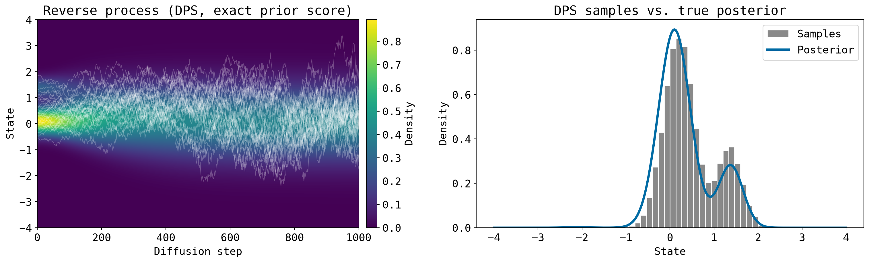
Although the learned prior was a good approximation of the true prior, we see that there is a clear mismatch between the learned and true posterior distributions. The histogram appears to be slightly shifted to the right. This can likely be exampled by the fact that the DPS approximation is not very accurate for the multimodal prior. We therefore need a more accurate training-free guidance method, which guarantees convergence to the true posterior distribution.

Twisted Diffusion Sampling

Twisted Diffusion Sampling (TDS) (Wu et al. 2024) combines diffusion guidance with Sequential Monte Carlo (SMC). As in DPS, it uses a tractable approximation of the measurement likelihood to guide the reverse diffusion process. The difference is that TDS treats this guidance only as a proposal and corrects it using importance weights.

To describe the method, discretize the diffusion interval as \(0=t_0<\cdots<t_N=T\), and write \(\mathbf{x}_i=\mathbf{x}(t_i)\). The Markovian structure of the learned reverse process gives

\[ p_{\boldsymbol{\theta}}(\mathbf{x}_{0:N}\mid\mathbf{y}) =\frac{1}{p(\mathbf{y})}p(\mathbf{x}_N) \prod_{i=0}^{N-1}p_{\boldsymbol{\theta}}(\mathbf{x}_i\mid\mathbf{x}_{i+1}) p(\mathbf{y}\mid\mathbf{x}_0). \tag{6}\]

The posterior \(p(\mathbf{x}_0\mid\mathbf{y})\) is the marginal of this distribution at \(t_0=0\). In SMC, we represent the distribution at each diffusion step by a weighted particle ensemble \(\{(\mathbf{x}_i^k,w_i^k)\}_{k=1}^K\), where \(\mathbf{x}_i^k\) is a state and \(w_i^k\) is its associated importance weight at time \(t_i\). Through a clever choice of the twisting function, we can ensure that the ensemble at time \(0\) approximates the true posterior \(p(\mathbf{x}_0\mid\mathbf{y})\).

A naive SMC sampler would propagate the particles using the full unconditional reverse process and only set the weights as \(w_0^k=p(\mathbf{y}\mid\mathbf{x}_0^k)\) at the final step. However, since most particles may reach \(t=0\) in regions where \(p(\mathbf{y}\mid\mathbf{x}_0)\) is negligible, this gives a small effective sample size and a poor approximation. TDS avoids this by introducing a twisting function

\[ \begin{aligned} \psi_i(\mathbf{x}_i) :=p(\mathbf{y}\mid X_0=\widehat{\mathbf{x}}_0(\mathbf{x}_i)) \approx p(\mathbf{y}\mid\mathbf{x}_i) =\int p(\mathbf{y}\mid\mathbf{x}_0) p(\mathbf{x}_0\mid\mathbf{x}_i)\,\mathrm{d}\mathbf{x}_0, \end{aligned} \tag{7}\]

which approximates the likelihood of the observation at intermediate diffusion times. In the same way as DPS, the intractable likelihood \(p(\mathbf{y}\mid\mathbf{x}_i)\) is approximated using Tweedie’s formula. At the final step no approximation is required, so we set \(\psi_0(\mathbf{x}_0)=p(\mathbf{y}\mid\mathbf{x}_0)\).

Replacing the measurement-alignment term in Equation 5 with the gradient of the twisting function, we obtain the approximate conditional score

\[ \widetilde{\mathbf{s}}(\mathbf{x}_i,t_i) =\mathbf{s}_{\boldsymbol{\theta}}(\mathbf{x}_i,t_i) +\nabla_{\mathbf{x}_i}\log\psi_i(\mathbf{x}_i). \tag{8}\]

Substituting this into the discretized reverse SDE from Equation 4 gives a proposal \(q_i(\cdot\mid\mathbf{x}_{i+1},\mathbf{y})\) which pushes particles towards states that are both likely under the learned prior and compatible with the observations. The crucial difference from DPS is that TDS corrects for sampling from \(q_i\) rather than from the original reverse transition. By initializing

\[ \mathbf{x}_N^k\overset{\mathrm{iid}}{\sim}p_T, \qquad w_N^k=\psi_N(\mathbf{x}_N^k), \qquad k=1,\ldots,K, \]

the ensemble is corrected at a generic step from \(t_{i+1}\) to \(t_i\) by first computing the normalized weights

\[ \dot{w}_{i+1}^k =\frac{w_{i+1}^k}{\sum_{j=1}^K w_{i+1}^j}. \]

We then resample \(K\) parent particles according to these weights,

\[ \dot{\mathbf{x}}_{i+1}^k \sim\sum_{j=1}^K\dot{w}_{i+1}^j\delta_{\mathbf{x}_{i+1}^j}, \qquad k=1,\ldots,K, \]

where \(\delta_{\mathbf{x}}\) denotes a point mass at \(\mathbf{x}\). Thus, particles with large weights may be selected several times, while particles with small weights may disappear from the ensemble. Each resampled parent is then propagated using the twisted proposal,

\[ \mathbf{x}_i^k\sim q_i(\cdot\mid\dot{\mathbf{x}}_{i+1}^k,\mathbf{y}). \]

Since this proposal differs from the original reverse transition, the propagated particle receives the incremental importance weight

\[ w_i^k =\frac{ p_{\boldsymbol{\theta}}(\mathbf{x}_i^k\mid\dot{\mathbf{x}}_{i+1}^k) \psi_i(\mathbf{x}_i^k) }{ q_i(\mathbf{x}_i^k\mid\dot{\mathbf{x}}_{i+1}^k,\mathbf{y}) \psi_{i+1}(\dot{\mathbf{x}}_{i+1}^k) }. \tag{9}\]

The procedure then repeats by normalizing the new weights, resampling the particles, propagating them one step, and computing the next set of weights until we reach \(i=0\).

The role of the correction in Equation 9 can be seen by multiplying the proposal densities and importance weights along a trajectory

\[ \begin{aligned} p(\mathbf{x}_N)\psi_N(\mathbf{x}_N) \prod_{i=0}^{N-1} \left[ q_i(\mathbf{x}_i\mid\mathbf{x}_{i+1},\mathbf{y}) \frac{ p_{\boldsymbol{\theta}}(\mathbf{x}_i\mid\mathbf{x}_{i+1})\psi_i(\mathbf{x}_i) }{ q_i(\mathbf{x}_i\mid\mathbf{x}_{i+1},\mathbf{y})\psi_{i+1}(\mathbf{x}_{i+1}) } \right] =p(\mathbf{x}_N) \prod_{i=0}^{N-1}p_{\boldsymbol{\theta}}(\mathbf{x}_i\mid\mathbf{x}_{i+1}) p(\mathbf{y}\mid\mathbf{x}_0). \end{aligned} \]

The proposal densities cancel, as do the intermediate twisting functions. What remains is exactly the unnormalized target in Equation 6. Consequently, the intermediate \(\psi_i\) only affect how efficiently particles are proposed; they do not change the SMC target. Under the conditions given by Wu et al. (2024), the particle approximation converges to the posterior of the discretized diffusion model as \(K\to\infty\).

Implementing the TDS algorithm, we replace the DPS guidance term with the gradient of the twisting function and compute the importance weights according to Equation 9. The following code illustrates this procedure and compares the learned and true posterior distributions.

def log_twisting_function(
    x_t: Array,
    i: int,
    integrated_betas: Array,
    score_function: Callable[[Array, int], Array],
    observation: float,
    observation_std: float,
) -> Array:
    if i == 0:
        x_0_hat = x_t
    else:
        x_0_hat = tweedie_mean(x_t, i, integrated_betas, score_function)
    return stats.norm.logpdf(observation, x_0_hat, observation_std)


def systematic_resample(key: Array, normalized_weights: Array) -> Array:
    num_particles = len(normalized_weights)
    offset = random.uniform(key) / num_particles
    positions = offset + jnp.arange(num_particles) / num_particles
    return jnp.searchsorted(jnp.cumsum(normalized_weights), positions)


def sample_tds(
    key: Array,
    initial_particles: Array,
    betas: Array,
    dt: float,
    integrated_betas: Array,
    score_function: Callable[[Array, int], Array],
    observation: float,
    observation_std: float,
) -> tuple[Array, Array, Array]:
    num_steps = len(betas)
    num_particles = len(initial_particles)
    particles = initial_particles
    particle_history = [particles]
    ancestor_history = []

    log_weights = log_twisting_function(
        particles,
        num_steps,
        integrated_betas,
        score_function,
        observation,
        observation_std,
    )

    for i in range(num_steps, 0, -1):
        key, resampling_key, proposal_key = random.split(key, 3)
        ancestor_indices = systematic_resample(resampling_key, softmax(log_weights))
        x_t = particles[ancestor_indices]

        prior_score = score_function(x_t, i)
        alignment = measurement_alignment(
            x_t,
            i,
            integrated_betas,
            score_function,
            observation,
            observation_std,
        )
        twisted_score = prior_score + alignment

        beta_t = betas[i - 1]
        transition_std = g(beta_t) * jnp.sqrt(dt)
        prior_mean = x_t - (f(x_t, beta_t) - g(beta_t) ** 2 * prior_score) * dt
        proposal_mean = x_t - (f(x_t, beta_t) - g(beta_t) ** 2 * twisted_score) * dt
        particles = proposal_mean + transition_std * random.normal(
            proposal_key, shape=x_t.shape
        )

        log_twist_t = log_twisting_function(
            x_t,
            i,
            integrated_betas,
            score_function,
            observation,
            observation_std,
        )
        log_twist_previous = log_twisting_function(
            particles,
            i - 1,
            integrated_betas,
            score_function,
            observation,
            observation_std,
        )
        log_weights = (
            stats.norm.logpdf(particles, prior_mean, transition_std)
            + log_twist_previous
            - stats.norm.logpdf(particles, proposal_mean, transition_std)
            - log_twist_t
        )

        particle_history.append(particles)
        ancestor_history.append(ancestor_indices)

    # Follow the resampling indices backwards so plotted lines are particle paths,
    # rather than connections between unrelated particles in adjacent populations.
    lineage_indices = jnp.arange(num_particles)
    trajectories = [particle_history[-1]]
    for i in range(num_steps - 1, -1, -1):
        lineage_indices = ancestor_history[i][lineage_indices]
        trajectories.append(particle_history[i][lineage_indices])

    normalized_weights = softmax(log_weights)
    return key, jnp.stack(trajectories), normalized_weights


key, initial_key = random.split(key)
initial_particles = random.normal(initial_key, shape=(num_samples,))
key, tds_trajectories, tds_weights = sample_tds(
    key,
    initial_particles,
    betas,
    dt,
    integrated_betas,
    exact_prior_score,
    observation,
    observation_std,
)

plot_reverse_samples(
    tds_trajectories,
    posterior_density_by_time,
    posterior_density,
    "Reverse process (TDS, exact prior score)",
    "TDS samples vs. true posterior",
    "Posterior",
    sample_weights=tds_weights,
)

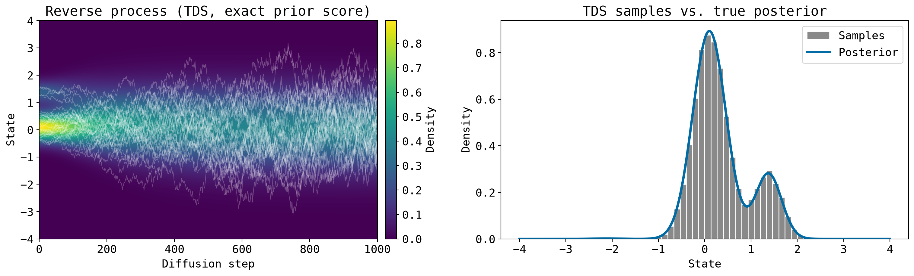
Compared to DPS, TDS gives a much better approximation of the posterior distribution, and the critical statistician is likely happier with the result.

Thank you for reading! If you have any questions or comments, feel free to reach out.

References

Anderson, Brian D. O. 1982. “Reverse-Time Diffusion Equation Models.” Stochastic Processes and Their Applications 12 (3): 313–26. https://doi.org/10.1016/0304-4149(82)90051-5.

Chung, Hyungjin, Jeongsol Kim, Michael T. Mccann, Marc L. Klasky, and Jong Chul Ye. 2024. Diffusion Posterior Sampling for General Noisy Inverse Problems. arXiv. https://doi.org/10.48550/arXiv.2209.14687.

Dunson, D. B., and J. E. Johndrow. 2020. “The Hastings Algorithm at Fifty.” Biometrika 107 (1): 1–23. https://doi.org/10.1093/biomet/asz066.

Lai, Chieh-Hsin, Yang Song, Dongjun Kim, Yuki Mitsufuji, and Stefano Ermon. 2025. The Principles of Diffusion Models. arXiv. https://doi.org/10.48550/arXiv.2510.21890.

Song, Yang, Jascha Sohl-Dickstein, Diederik P. Kingma, Abhishek Kumar, Stefano Ermon, and Ben Poole. 2021. Score-Based Generative Modeling Through Stochastic Differential Equations. arXiv. https://doi.org/10.48550/arXiv.2011.13456.

Wu, Luhuan, Brian L. Trippe, Christian A. Naesseth, David M. Blei, and John P. Cunningham. 2024. Practical and Asymptotically Exact Conditional Sampling in Diffusion Models. arXiv. https://doi.org/10.48550/arXiv.2306.17775.